R Shiny How to Read Table Inputand Render Table Output Example
Getting Started with R Shiny
Have the first steps towards becoming an R shiny expert

Intro to R Shiny
Shiny is an R parcel that allows programmers to build web applications within R. For someone like me, who plant building GUI applications in Coffee really hard, Shiny makes it much easier.
This blog commodity will get you edifice Shiny apps straight away with working examples. Showtime things get-go, make certain you lot install the shiny package.
install.packages("shiny") Shiny App Structure
Like R files, Shiny apps also end with a .R extension. The app structure consists of three components, which are:
- A user interface object (ui)
- A server function
- A role call to shinyApp
The user interface (ui) o bject is used to manage the appearance and layout of the app, such as radio buttons, panels, and option boxes.
# Ascertain UI for app
ui <- fluidPage(# App championship ----
titlePanel("!"),# Sidebar layout with input and output definitions ----
sidebarLayout(# Sidebar console for inputs
sidebarPanel()
# Allow user to select input for a y-axis variable from drop-down
selectInput("y_varb", label="Y-axis variable",choices=names(data)[c(-ane,-three,-4)]), # Output: Plot
("plot", dblclick = "plot_reset") )
The server function contains data that is required to build the app. This includes instructions to generate a plot or table and react to user clicks for example.
# Ascertain server logic here ----
server <- function(input, output) {# 1. It is "reactive" and therefore updates 10-variable based on y- variable selection
# 2. Its output type is a plot
output$distPlot <- renderPlot({ remaining <- reactive({
names(data)[c(-ane,-3,-4,-match(input$y_varb,names(data)))]
})observeEvent(remaining(),{
choices <- remaining()
updateSelectInput(session = getDefaultReactiveDomain(),inputId = "x_varb", choices = choices)
})}
output$plot <- renderPlot({
#ADD YOUR GGPLOT CODE Hither
subset_data<-data[1:input$sample_sz,]
ggplot(subset_data, aes_string(input$x_varb, input$y_varb))+
geom_point(aes_string(colour=input$cat_colour))+
geom_smooth(method="lm",formula=input$formula) }, res = 96)
}
Lastly, the shinyApppart builds Shiny app objects based on the UI/server pair.
          library(shiny)
            # Build shiny object
            shinyApp(ui = ui, server = server)
            # Phone call to run the application
runApp("my_app")
What is Reactivity?
Reactivity is all about linking user inputs to app outputs; so that the display in the Shiny app is dynamically updated based on user input or selection.
The edifice blocks of reactive programming
Input
The input object, which is passed to the shinyServeroffice allows the user to access the app'due south input fields. Information technology is a list-like object that contains all the input data sent from the browser, named according to the input ID.
Unlike a typical list, input objects are read-only. If you lot effort to modify an input inside the server function, you'll get an error. The input can only be set by the user. This is done by creating a reactive expression, where a normal expression is passed into reactive. To read from an input, you must be in a reactive context created by a role like renderText() or reactive().
Output
To allow reactive values or inputs to exist viewed in an app, they need to be assigned to the output object. Like the input object, it is likewise a list-similar object. It typically works with a renderrole like renderTable.
The renderfunction performs the following ii operations:
- It sets upward a reactive context that is used to automatically associate inputs with outputs.
- It converts the R lawmaking output into HTML lawmaking to allow it to be displayed on an app.
Reactive Expressions
Reactive expressions are used to split the code within the app into sizeable lawmaking chunks that not only reduce code duplication but also avoid re-computation.
In the below instance, the reactive code receives four inputs from the user, which are then used to output results from an independent-samples t-test.
server <- function(input, output) { x1 <- reactive(rnorm(input$n1, input$mean1, input$sd1)) x2 <- reactive(rnorm(input$n2, input$mean2, input$sd2)) output$ttest <- renderPrint({ t.test(x1(), x2()) }) }
Shiny App Examples
Now, that we know some basics let'due south build some apps.
App One
The app uses a dummy dataset that includes three continuous variables. The requirements for the app are as follows:
- Produce a scatterplot between two of the iii continuous variables in the dataset, where the first variable can't be graphed against itself.
- User tin can select the x and y-variables for plotting
- User can select the formula for plotting ("y~ten", "y~poly(ten,2)", "y~log(x)").
- The chiselled variable selected is used to colour the points the scatterplot
- The user can select the number of rows (sample size), ranging from 1 to 1,000 for plotting.
#Load libraries
library(shiny)
library(ggplot2) #Create dummy dataset
thousand<-1000
set.seed(999)
data<-data.frame(id=i:one thousand)
data$gest.age<-round(rnorm(chiliad,34,.v),1)
data$gender<-factor(rbinom(k,1,.5),labels=c("female","male"))
z = -ane.5+((((information$gest.age-hateful(data$gest.age)))/sd(data$gest.age))*-1.v)
pr = 1/(1+exp(-z))
information$mat.smoke = factor(rbinom(thou,1,pr))
data$bwt<- round(-iii+data$gest.age*0.15+
((as.numeric(data$mat.smoke)-1)*-.1)+
((every bit.numeric(data$mat.smoke)-1))*((data$gest.historic period*-0.12))+
(((as.numeric(data$mat.smoke)-1))*(4))+
((as.numeric(data$gender)-1)*.ii)+rnorm(k,0,0.i),3)
data$mat.bmi<-round((122+((data$bwt*x)+((data$bwt^8)*2))/200)+
rnorm(one thousand,0,ane.5)+(data$gest.age*-3),1) rm(z, pr, m) #Define UI
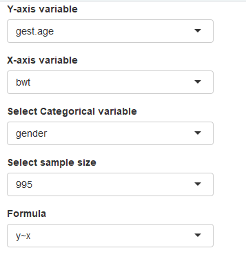
ui <- fluidPage(#1. Select 1 of 3 continuous variables as y-variable and x-variable
#2. Colour points using categorical variable (1 of 4 options)
selectInput("y_varb", label="Y-axis variable",choices=names(data)[c(-1,-three,-4)]),
selectInput("x_varb", label="10-axis variable", choices=NULL),
selectInput("cat_colour", characterization="Select Chiselled variable", choices=names(data)[c(-1,-2,-5,-half-dozen)]), #three. Select sample size
selectInput("sample_sz", label = "Select sample size", choices = c(ane:1000)),
#iv. Three unlike types of linear regression plots
selectInput("formula", label="Formula", choices=c("y~x", "y~poly(x,two)", "y~log(x)")),
#5. Reset plot output after each selection
plotOutput("plot", dblclick = "plot_reset"))
server <- function(input, output) {#one. Register the y-variable selected, the remaining variables are at present options for x-variable
remaining <- reactive({
names(information)[c(-ane,-3,-four,-lucifer(input$y_varb,names(data)))]
})observeEvent(remaining(),{
choices <- remaining()
updateSelectInput(session = getDefaultReactiveDomain(),inputId = "x_varb", choices = choices)
})output$plot <- renderPlot({
}, res = 96)
#Produce scatter plot
subset_data<-information[ane:input$sample_sz,]
ggplot(subset_data, aes_string(input$x_varb, input$y_varb))+
geom_point(aes_string(colour=input$cat_colour))+
geom_smooth(method="lm",formula=input$formula)
} # Run the application
shinyApp(ui = ui, server = server)
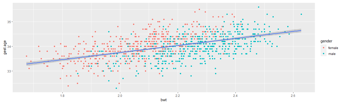
Once the user has selected the inputs, the scatter plot below is generated.
There you lot become, that'due south your offset spider web app built. However, let's break the code downwards further.
App One Explanation
The part selectInputis utilised to brandish the driblet-down menus for a user to select the variables for plotting, the variable for colouring the points in the scatter plot, and the sample size.
Within the serveroffice, based on the user'due south selection for the y-variable, the user's choices are updated for the 10-variable. The observeEventfunction is used to perform an action in response to an event. In this example, it updates the listing of x-variables that can be selected for the ten-centrality; so that the same variable can not be plotted on both the y-centrality and the x-axis.
The function renderPlotis then used to take all the inputs, 10-variable, y-variable, categorical-variable, sample size, and formula to generate or 'return' a plot.
In that location you have it, your commencement Shiny App.
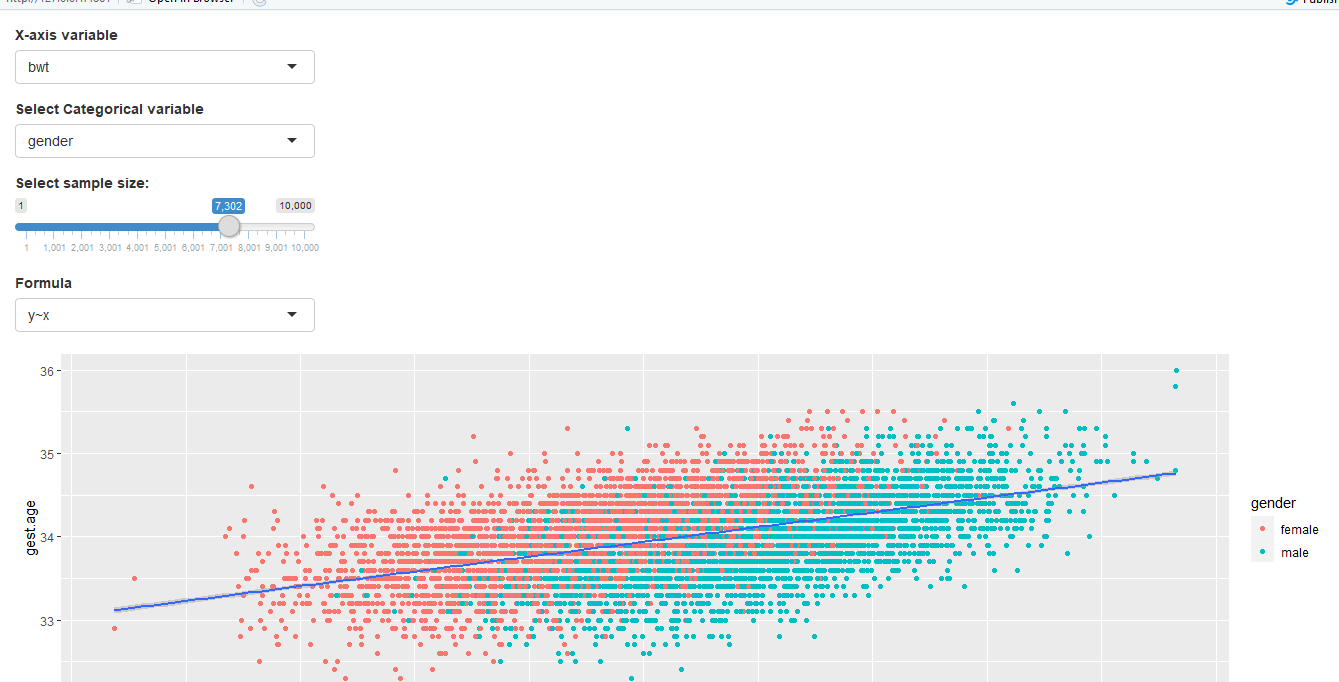
At present, what if we wanted the drop-down to be a slider instead. You can modify the code by adding this code snippet in.
          ui <- fluidPage(                 #three. Select sample size
              # numericInput("sample_sz", "Input sample size", 10000),
              sliderInput(inputId = "sample_sz",
              label = "Select sample size:",
              min = 1,
              max = 10000,
              value = 1)
)
The output will then await similar what's displayed in
Now, allow's move onto the next example which is slightly more than complicated.
App Two
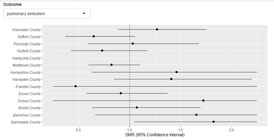
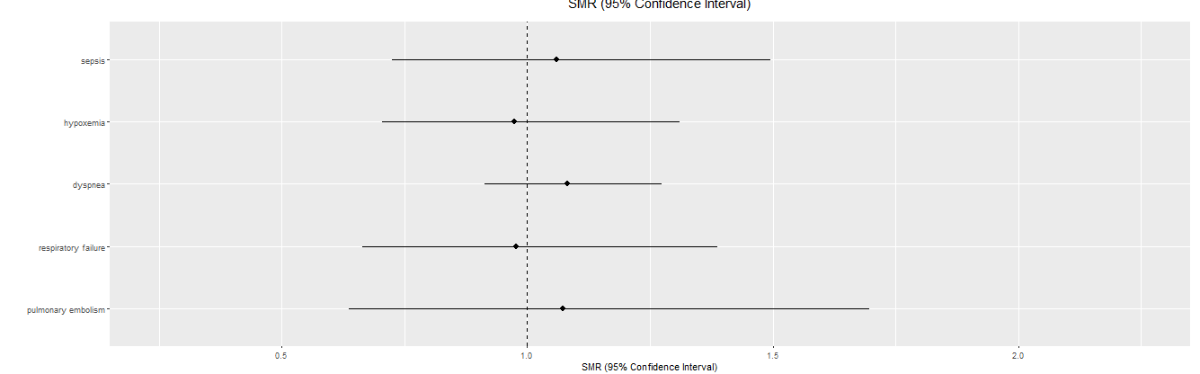
In this app, we are looking at a dataset that looks at five life-threatening outcomes equally a upshot of the COVID-xix infection. Nosotros want the app to do the following:
- Let the user to select one of the five outcomes as an input
- Compare the different counties by the selected event in a forest plot
- If a user selects a county in the plot, then some other forest plot should be generated that shows all five outcomes for the selected state.
- Display an error message for missing values.
#Load libraries
library(shiny)
library(ggplot2)
library(exactci) #import the data and restrict the data to variables and patients of interestpatient.data<-read.csv("Synthea_patient_covid.csv", na.strings = "")
#Become the state average for each outcome
cons.data<-read.csv("Synthea_conditions_covid.csv", na.strings = "")
information<-merge(cons.information, patient.data)
information<-data[which(information$covid_status==ane),]
data<-data[,c(12,14,65,96,165,194)]
country.average<-employ(data[,-6],MARGIN=two,FUN=mean) #Make better names for the outcomes
names<-c("pulmonary embolism", "respiratory failure", "dyspnea", "hypoxemia", "sepsis") #Calculate and aggregate the obs and exp by outcome and county
data$sample.size<-one
listing<-list()
for (i in 1:5) {
list[[i]]<-cbind(upshot=rep(names[i],length(unique(data$COUNTY))),
amass(data[,i]~County, sum,data=data),
exp=round(aggregate(sample.size~COUNTY, sum,data=data)[,2]
*state.average[i],2))
}
plot.data<-practise.call(rbind,list)
names(plot.data)[3]<-"obs" #Lastly, obtain the smr (called est), lci and uci for each row
#Add conviction limits
plot.information$est<-NA
plot.data$lci<-NA
plot.data$uci<-NA
#Summate the confidence intervals for each row with a for loop and add them to the plot.data
for (i in 1:nrow(plot.information)){
plot.data[i,5]<-as.numeric(poisson.verbal(plot.information[i,3],plot.information[i,4],
tsmethod = "central")$judge)
plot.data[i,6]<-as.numeric(poisson.exact(plot.data[i,3],plot.data[i,4],
tsmethod = "cardinal")$conf.int[i])
plot.information[i,7]<-as.numeric(poisson.exact(plot.data[i,3],plot.information[i,iv],
tsmethod = "primal")$conf.int[two])
} # Define UI for application
ui <- fluidPage(
selectInput("outcome_var", characterization="Outcome",unique(plot.data$event)),
plotOutput("plot", click = "plot_click"),
plotOutput("plot2")
)
server <- function(input, output) {output$plot <- renderPlot({
#Output fault message for missing values
validate(
need( nrow(plot.data) > 0, "Data insufficient for plot")
)
ggplot(subset(plot.data,outcome==input$outcome_var), aes(ten = COUNTY,y = est, ymin = pmax(0.25,lci),
ymax = pmin(2.25,uci))) +
geom_pointrange()+
geom_hline(yintercept =1, linetype=two)+
coord_flip() +
xlab("")+ ylab("SMR (95% Confidence Interval)")+
theme(legend.position="none")+ ylim(0.25, 2.25)
}, res = 96)#Output error message for missing values
#modify this plot so information technology's the aforementioned forest plot as above but shows all outcomes for the selected cantonoutput$plot2 <- renderPlot({
validate(
need( nrow(plot.data) > 0, "Data insufficient for plot as it contains a missing value")
)
#Output error message for trying to circular a value when it doesn't exist/missing
validate(
need( as.numeric(input$plot_click$y), "Not-numeric y-value selected")
)forestp_data<-plot.data[which(plot.data$COUNTY==names(table(plot.data$Canton))[round(input$plot_click$y,0)]),]
ggplot(forestp_data, aes(x = outcome,y = est, ymin = pmax(0.25,lci), ymax = pmin(two.25,uci))) +
geom_pointrange()+
geom_hline(yintercept =one, linetype=2)+
coord_flip() +
xlab("")+ ylab("SMR (95% Confidence Interval)")+
theme(legend.position="none")+ ylim(0.25, ii.25)
})}
# Run the awarding
shinyApp(ui = ui, server = server)
App Ii Caption
In this app, similar App One, the user makes a option for an event from the drop-down box. This results in a forest plot. The calculations for this forest plot are done outside of the Shiny user interface. The tricky bit in this application is to build a reactive 2d plot in response to the user clicked county in the first plot.
This reactivity happens in the server function using this line
plot.data[which(plot.data$COUNTY==names(table(plot.data$Canton))[circular(input$plot_click$y,0)]),] where nosotros checked to run across which county had been selected in club to display the second forest plot for all v outcomes.
In the app, an fault message is displayed using the validaterole where if at that place is missing data, then at that place is an error displayed due to this piece of syntax:
[round(input$plot_click$y,0)],]
App Three
The concluding spider web app'due south objective is to let the user to plot the relationship betwixt the variables in the information gear up. Some variables are categorical, while others are continuous. When plotting ii continuous variables, the user should just exist able to plot them on a scatter plot. When ane continuous variable and i chiselled variable is selected, the user should only exist able to make a box plot. The user should not be able to brand a plot with 2 categorical variables. The app should merely display 1 plot at a fourth dimension, based on the user'south selection.
#Load libraries
library(shiny)
library(ggplot2) #import data
setwd("C:/Users/User/Desktop/Synthea")
patient.information<-read.csv("Synthea_patient_covid.csv", na.strings = "")
obs.data<-read.csv("Synthea_observations_covid.csv", na.strings = "") patient.data$dob<-as.Date(patient.data$BIRTHDATE, tryFormats = "%d/%m/%Y")
patient.data$enc.date<-as.Date(patient.information$Appointment, tryFormats = "%d/%k/%Y")
patient.information$age<-as.numeric((patient.data$enc.date-patient.data$dob)/365.25)
information<-merge(obs.data, patient.data)
data<-na.omit(data[,c(iv,5,10:12,20,24,32,18,xv,23,31,33,48:51,sixty)])
names(data)<-substr(names(data),1,10)
information$covid_stat<-as.factor(information$covid_stat)
information$dead<-as.cistron(data$dead) # Define UI for application
ui <- fluidPage(
#1. Select 1 of many continuous variables every bit y-variable
selectInput("y_varb", label="Y-centrality variable",choices=names(data)[c(-one,-two,-14,-15,-sixteen,-17)]),#2 Select whatsoever variable in dataset as x-variable
selectInput("x_varb", label="X-axis variable", choices=names(data)),#iii. Reset plot1 output subsequently each choice
)
plotOutput("plot", dblclick = "plot_reset")
server <- function(input, output) {remaining <- reactive({
names(data)[-match(input$y_varb,names(data))]
})observeEvent(remaining(),{
choices <- remaining()
updateSelectInput(session = getDefaultReactiveDomain(),inputId = "x_varb", choices = choices)
})output$plot <- renderPlot({
if ( is.numeric(information[[input$x_varb]]) ) {
ggplot(data, aes_string(input$x_varb, input$y_varb)) + geom_point()
} else {
ggplot(data, aes_string(input$x_varb, input$y_varb)) + stat_boxplot()
} })}
# Run the application
shinyApp(ui = ui, server = server)


App Iii Caption
The catchy bit in this app is using the if-else condition inside renderPlotand then that only i of the ii types of plots (scatter plot or box plot) tin be selected. Furthermore, when y'all want to check the class of the input$x_varb the use of double square brackets (list) is required, information[[input$x_varb]],otherwise the output will always be character.
Conclusion
So, there you accept it, three simple apps. Let'due south recap very rapidly on what was covered in this blog article.
- Structure of an R Shiny app
- Linking inputs and outputs
- Creating a dynamic user interface by using reactive() and observeEvent
- Displaying mistake letters using validate
Source: https://towardsdatascience.com/getting-started-with-r-shiny-821eb0328e73
0 Response to "R Shiny How to Read Table Inputand Render Table Output Example"
Publicar un comentario